Review on the Recent Welding Research with Application of CNN-Based Deep Learning Part I: Models and Applications
합성곱 신경망기반 딥러닝의 용접연구 적용 Part I: 모델과 활용사례
Article information

Abstract
During machine learning algorithms, deep learning refers to a neural network containing multiple hidden layers. Welding research based upon deep learning has been increasing due to advances in algorithms and computer hardwares. Among the deep learning algorithms, the convolutional neural network (CNN) has recently received the spotlight for performing classification or regression based on image input. CNNs enables end-to-end learning without feature extraction and in-situ estimation of the process outputs. In this paper, 18 recent papers were reviewed to investigate how to apply CNN models to welding. The papers was classified into 5 groups: four for supervised learning models and one for unsupervised learning models. The classification of supervised learning groups was based on the application of transfer learning and data augmentation. For each paper, the structure and performance of its CNN model were described, and also its application in welding was explained.
1. Introduction
Deep learning is one of the machine learning techniques, a kind of Artificial Intelligence (AI), with increasing applications to a wide range of sectors. Machine learning is not based on explicit rules, it learns rules using datasets, and is categorized into supervised learning, unsupervised learning, and reinforcement learning according to the types of training datasets. Supervised learning uses inputs and correct outputs as training datasets and it is applied to classification and regression problems1).
Artificial Neural Network (ANN), a type of machine learning, was developed by mimicking human neural networks and consists of an input layer, hidden layers, and an output layer. ANN is further categorized into a shallow neural network (SNN) where there is one hidden layer and a deep neural network (DNN) where there are two or more hidden layers. When machine learning is performed using DNN, it is called deep learning.
As for research that applies ANN to welding, since the error back-propagation algorithm2) was introduced in the mid-1980s, ANN has been actively applied to a number of welding processes. The examples of application includes prediction of weld quality from control parameters3,4), suggestion of appropriate control welding parameters from the welding of the desired weld attributes5), profile extraction from laser vision sensing image6), and quality and seam tracking using vision sensors7). However, there were some problems in expanded application of neural network models at the time. First, the sigmoid function or RBF (Radial Basis Function) function was mainly used as an activation function of neural networks, and learning of weights far from the output layers was difficult in training of DNN through the back-propagation algorithm. In addition, when images or time series signals were used, learning was performed through feature extraction rather than raw signals without feature extraction, and models that predict outputs from scalar variables such as control parameters were mainly developed, and thus application of the trained model to another production system was intrinsically difficult. When only the control parameters are used as the input parameters of the model, several environmental disturbances (e.g. humidity, temperature, electric power instability) cannot be considered, and it was difficult to set the same system inputs even by setting the same control parameters in other systems.
In recent years, ReLu (Rectified Linear unit) has been proposed as an activation function to enable training of DNN. With the introduction of Convolutional Neural Networks (CNNs)8), also known as convnets, which are mainly used for image recognition, and Recurrent Neural Network (RNN)9,10) for use in models using time-series variables, innovative development in deep learning technologies has been achieved including end- to-end learning.
Machine learning has been applied to various welding processes and the examples include the use of deep learning and reinforcement learning in the laser welding control11), quality prediction through deep learning in arc welding12), and quality classification through SVM (Supported Vector Machine), a machine learning algorithim 13,14).
In this paper, 18 recently published papers on CNN- based welding research are reviewed. As shown in Fig. 1, these papers were divided into 5 groups based on supervised/unsupervised learning, use of transfer learning, and application of data augmentation in data preprocessing.
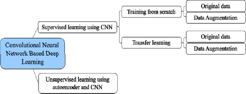
Classification of papers reviewed
2. CNN Structure and Learning Methods
CNN is an artificial neural network that uses convolution operations, and CNN models has shown excellent performance in image recognition because the feature patterns of the images can be extracted by training through convolutional filters. In addition, manual extraction of features is not necessary since features are automatically learned, and models can be constructed based on pre-trained networks. With these advantages, research of applying CNNs for deep learning using images has shown a rapid increase in recent years.
2.1 Basic structure
CNN is composed of convolutional layers, pooling layers, and fully connected layers. In the convolutional layer, inputs within a kernel are connected by specific weights, and a feature map is constructed by information representing each kernel area and passed to the next layer. The convolution operation is performed by sliding the kernel window over the input data at a fixed stride. The output of the convolutional layer can be passed to the next layer as it is, but in most cases, pooling is performed, one of the down sampling operation, to prevent over-fitting and create features that are highly noise-resistant. Typical pooling methods are max pooling and mean pooling, in which the maximum and mean values are output within the specified kernel window, respectively. The fully connected layer is a layer in which nodes of the previous layer and those of the next layer are all connected in the same way as a traditional ANN. In the CNN model, the successive repetition of the convolutional layer and the pooling layer enables inclusion of local features in the image and also represents the global features and these are passed as the input of the fully connected layer, and the fully connected layer produces the final output.
2.2 Key techniques used in the reviewed papers
The techniques adopted for modeling and training are briefly introduced as follows, and more details can be found in References15).
2.2.1 Activation function
The activation function converts the input signal of a node in an ANN to an output signal, and the identity function, sigmoid, Tanh, ReLu, and softmax function are used as the activation function. In general, ANN performs learning of complex nonlinear phenomena by adopting a nonlinear function as an activation function. Among them, the sigmoid function is useful for converting all values into probabilities, and generates output values between 0 or 1, which can be used for binary classification. The Tanh function has a smooth shape like the sigmoid function, and has the advantage of being able to generate negative values because the output values range between -1 and 1 depending on the input value. The sigmoid function and the tanh function are disadvantageous for use in the learning of DNN because it is possible that the gradient of the function vanishes by saturation. However, the ReLU function outputs 0 when the input value is negative, and outputs the input value as it is when the input is 0 or positive. The softmax function used in the classification problem converts the input values between 0 and 1 and the sum of the output values is always 1. The softmax function increases the differences in the portions of the input values, making the portion of the largest value even larger and the portions of other values even smaller, and is used as the activation function of the last node for the classification neural network.
2.2.2 Transfer learning
Transfer learning performs learning by using models that has been pre-trained with large-scale data such as VGG, GoogLeNet, and MobileNet, rather than learning a complex CNN structure from scratch in the design of an image classification model using CNN and it allows a accurate model in a relatively time-efficient manner. Transfer learning adopts model optimization through fine-tuning. The fine-tuning strategies can be divided into three methods: retraining the entire model, fine- turning only the parameters of the fully connected (FC) layers, and fine-tuning some convolutional layers and all fully connected layers.
2.2.3 Data augmentation
In deep learning, the more number of training datasets are available, improved accuracy can be achieved. Insufficient number of training datasets leads to over- fitting and ensuring a large number of training datasets is important in the performance. When CNN uses images as input data and the number of training datasets is insufficient, data augmentation can be used to address the problem of insufficient input. Data augmentation is a method of adding artificially processed images to the given training datasets through effects such as flipping, rotation, and changing brightness to the input images. In this paper, for convenience of presentation, the method of using original data without data augmentation is indicated as learning using the original data.
3. Supervised learning with training from scratch
3.1 Original data utilization
Z. Guo et al.16) proposed a model for classifying normal and defective welds by applying CNN to electric resistance welding in the line pipe manufacturing process, and achieved an accuracy of 99.01%. The cross-section images of the welds were used as input and the sigmoid function was used in the output layer to classify normal and defective welds. The number of hidden layers of the CNN was 5, 7, and 13, and the difference in accuracy according to the network depth was examined. With increasing network depth, the average time per epoch was 261.68 s, 266.24 s, and 267.26 s in case of 5, 7, and 13 layers, respectively, indicating no significant difference but the error rates were 7.89%, 4.93%, and 0.99%, showing improved accuracy. It was reported that superior accuracy results were obtained compared to the error rate of 2.3% at human inspection.
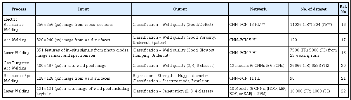
Summary of research using original data and training from scratch
A. Kjumaidi et al.17) proposed a CNN-based defect detection model using photo images of arc welding bead surface as input, and using only 3 hidden CNN layers and 2 hidden FC layer, test accuracy of 95.83% was achieved for 4-class classification of defects (good, porosity, undercut, and spatter).
Y. Zhang et al.18) performed in-situ measurement of welding signals using multi-sensor technology, and a CNN-based defect detection model was proposed based on the input signals. The multi-sensor system comprised a photodiode, a spectrometer, and two high-speed cameras. The collected photodiode signals were decomposed for each frequency by the Wavelet Packet Decomposition (WPD) method to obtain 320 feature signals. In addition, the spectrometer signals were collected by dividing the wavelength range between 400 nm and 900 nm into 25 bands. The information on the size and location of the keyholes was collected with No. 1 camera with 976 nm laser light and the bandpass filter applied, and the spatter and plume related information was collected from No. 2 camera with a wavelength range of 320 nm-750 nm. After collecting a total of 351 signals from various sensors at a frequency of 500 Hz, the rest were filled with value 1 to form 400 input nodes. For verification on the accuracy of the CNN model, the results were compared with the fully connected network (FCN) model19) result with same input nodes. In the comparison, the mean error of the FCN model was 9.65% and the mean error of the CNN model was 4.7%, indicating that the CNN model accuracy was superior to that of FCN model. For generalization of the proposed CNN model, the verification of the model was performed by experimenting under four welding conditions. As a result of CNN model classification, error rates of 1.73%, 8.0%, 11.2%, and 8.75% were obtained in each defect class (good, blowout, humping, undercut). When the cases of classification error were analyzed, there were cases where the blowout defect and the undercut defect were confused in detection, or the humping defect and good welds were confused.
D. Bacioiu et al.20) constructed various DNN models for welding defects classification in GTA welding of aluminum 5083 alloy and compared the model per- formances. In a total of 60 welding experiments, the in-situ molten pool images were used as input data, and the 6 CNN models and 6 FCN models were developed with defect classifications of 2-class (good, defective), 4-class (good, melt-through, contamination, lack of fusion) and 6-class (good, melt-through, contamination, lack of fusion, misalignment, lack of penetration). Then, the performance was compared according to input image resolution, model depth, and learning rate. In the evaluation of the input image resolution, the comparison of original data images of 800x974 pixels with sampled images at 400x487 and 25x30 pixels confirmed that in the 6-class classification the CNN model showed higher sensitivity to the final classification accuracy than the FCN model. In all models, the accuracy improved with increasing model depth, and learning did not converge at a learning rate of 10-3 or below. In all evaluations, CNN models showed higher accuracy than FCN models. S. Choi et al.21) presented a CNN model that predicts weld quality (tensile shear strength, nugget diameter, fracture mode of welds, expulsion occurrence) through the surface images of resistance spot welds for automobile steel sheets with a tensile strength of 980 MPa. The surface indentation and heat trace correlate with the weld quality, and thus the tensile shear strength, nugget diameter, fracture mode of welds, and expulsion occurrence were predicted with the accuracy of 98.6%, 98.8%, 100%, and 100%, respectively, through the CNN model. The generality of the model was verified through a test using data not included in the training, and the verification result confirmed that the prediction accuracy of the tensile shear strength and nugget diameter was 97.8% and 97.4%, respectively
Z. Zhang et al.22) used a CNN model to determine the penetration state of tailor-rolled blank (TRB) in-situ laser welding. The applied penetration state classification was 2-class (incomplete penetration, complete penetration), 3-class (incomplete penetration, desirable-complete penetration, overpenetration), and 4-class (incomplete penetration, desirable penetration, complete penetration, overpenetration). Six CNN models with different number of kernels and convolutional layers were trained and evaluated in comparison. It was confirmed that the increased complexity of the model did not necessarily lead to improved accuracy, and the optimal CNN model was determined considering the model complexity in addition to accuracy. Moreover, apart from the model complexity, the image sampling frequency (100 fps, 300 fps, 3000 fps) of the input images that can affect the latency of model was varied to conduct experiments in comparison. Since there was no significant difference in accuracy among models with difference sampling frequencies, 100 fps was selected with the lowest latency. To verify the applicability of the CNN model, it was compared with other methods [(HOG, LBP, Bag of features (BOF), or SAE)+SVM]. As a result of the verification, the CNN model in 2-class classification showed the highest prediction accuracy, and in the case of 3-class classification, the prediction accuracy of the CNN model was 99%, 93.8%, and 96.5%, respectively, indicating higher performance than other models.
When the penetration state was classified into 4 classes, the accuracy of each model was relatively low, but the stability in the accuracy of the CNN model was high.
3.2 Data augmentation
W. Hou et al.23) investigated a defect classification model (good, incomplete penetration, pore, slag inclusion, crack) from X-ray images of various welds in an open database GDXray. First, 3503 of 32×32-pixel images were extracted from 88 X-ray images by subsampling. Since the distribution of each type of defect is unbalanced, resampling was performed using ROS (Random Over Sampling), RUS (Random UnderSampling), and SMOTE (Synthetic Minority Oversampling TEchnique) methods. The RUS method is the simplest approach that randomly deletes samples from the majority class to balance the class distribution and the ROS method duplicates samples selected from the minority class and adds to the original dataset to balance the class distribution. In addition, the SMOTE method is a resampling method in which Euclidean distance is calculated to randomly find k-nearest neighbors to create new artificial samples. For classification models, traditional methods of Haralick texture features and HOG (Histograms of Oriented Gradients) were used as well as the deep learning method SSAE (Stacked Sparse Auto-Encoders), and two CNN models with different depths were used. For visual comparison on the results of extracted features through each model, each part was visualized into a 2D map using the t-SNE method to compare the accuracy. From the comparison, it was confirmed that the t-SNE map of the original images was disorderly, and the t-SNE map of the models with Haralick technique and HOG method also showed poor data classification performance. Both SSAE and CNN models showed better performance of classification in the t-SNE map. Between the two CNN models, the one with larger depth showed a better classification performance. Among them, the classification of samples without defects and samples with pores showed the best performance, and crack defects were the most difficult for classification. In the case of the ROS datasets, the mean accuracy of the defect classification for Haralick, HOG, SSAE, CNN1, and CNN2 was 60.9%, 81.6%, 91.4%, 94.7%, and 96.3%, respectively, in the case of the RUS datasets, the accuracy values were 60.7%, 67.5%, and 87.3. %, 76.6%, 79.9%, and for SMOTE datasets, the values were 63.1%, 82.2%, 90.5%, 94.4%, and 97.2%, respectively. In conclusion, they reported that the deep learning method showed better feature extraction performance than the traditional model, and that with SMOTE method, the problem of accuracy reduction from data imbalance can be resolved.
J. Park et al.24) proposed two-step CNN models for defect detection in engine transmission welds. In the first CNN model, the representation of collected images of the circular welding area of the engine transmission was converted from Polar coordinates to Cartesian coordinates and the center point was predicted. Assuming that the weld width was fixed, the background except the welds was removed, thereby optimizing the input data to the second defect detection CNN model. Compared with Hough circle, a traditional method, the two-step models have showed superior performance under dark lighting environments and with blurred images. Since there are not many defect data images in the training datasets, image transformation (rotation, translation, scaling) and image distortion (brightness and contrast adjustment) were performed to improve performance. In the second defect detection CNN model, the mini-batch gradient descent method can lead to biased learning due to data imbalance, class-specific batch sampling method with a set ratio of OK and NG images of each batch was used. For the defect detection model, the performance was comparatively evaluated between HOG+SVM, LBP (Local Binary Pattern)+SVM and four CNN models, and all CNN based models showed outstanding performances.

Summary of research using data augmentation and training from scratch
For automation of Flux Cored Arc (FCA) Welding, T. Ashida et al.25) used a CNN model to extract features of molten pool and calculated the distance between the leading of the molten pool and arc center and the width of the pool to investigate a feedback control system to form back bead. Data augmentation was performed using horizontal flip, translation, and scaling to increase the number of datasets from 2,400 to 12,000. When comparing between the proposed CNN model and the conventional feature-extraction image processing algorithms, the mean prediction error of the leading end position of the molten pool was reduced by 0.3 mm. The seam tracking and back bead formation was verified by implementing the developed feedback control algorithm to the butt weld joint with a joint gap from 3 mm to 10 mm along the weld seam which is also deviated by 10 mm from the pre-taught path.
Z. Zhang et al.26) developed a CNN model for in-situ weld defects prediction in pulsed gas tungsten arc (GTA) welding of aluminum alloys. In order to increase the training speed and accuracy of the CNN model, a system was devised to collect 3-way information simultaneously from the top front, top back, and back seam. Welding was performed on rectangular, dumbbell-shaped, and ladder-shaped specimens to generate welding defects. Downsampling was performed on the original images of 1392x1040 pixels with the arithmetic mean and thus input images of 100x100 pixels were used. For data augmentation, the number of datasets was increased by adding noise (salt and pepper noise) and randomly applying 15 and 30 degrees rotation to the input images. After the data augmentation, the accuracy improved by 3.88% from 92.3% to 96.18%, verifying the effectiveness of data augmentation. In addition, for optimization of CNN model, the accuracy and the final training speed were compared by varying 4 convolutional layer structures and the number of kernels. The training time and efficiency increased with the number of kernels, and the accuracy increased with the increase in the number of feature images excluding 2D images with only 0 in the pooling layer.
4. Supervised learning with transfer learning
4.1 Research using original data
H. Zhu et al.27) applied a CNN model for defects (normal, overlap, spatter, porosity) classification on weld surfaces of Gas Metal Arc Welding (GMAW). Transfer learning was performed using LeNet-5, and since the softmax function, which is frequently used in the last layer of the final fully connected layer of the CNN model, has a disadvantage of performance degradation when the number of training datasets is insufficient, Random Forest and SVM classifier were used for comparison of the performance. Preprocessing was performed such as median filtering, image enhancement by gradation processing, and OTSU image thresholding for all collected images of defects on weld surfaces. From the results obtained from softmax, SVM and Random Forest classifiers, the accuracy obtained using the softmax classifier was the lowest and the accuracy of the proposed Random Forest Classifier showed the best performance.
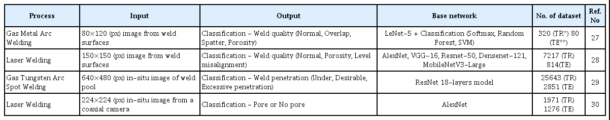
Summary of research using original data and transfer learning
Y. Yang et. al28) used photographs of laser welding area taken by CMOS digital camera and transfer learning of a CNN model was performed for classification of weld quality into 3 classes (normal, porosity, level misalignment) and 2 classes (qualified, defect). In the basic VGG-16 model, the weight of the convolutional layer was fixed and training was performed only on the weight of the FC layer. The result of this model was compared with the other eight models (pre-optimization AlexNet, Resnet- 50, VGG-16, Densenet-121, MobileNetV3-Large and post-optimization pre-AlexNet, pre-Resnet-50, and pre- Densenet-121). The 2-class binary classification achieved accuracy of 90% or higher in all cases. For multiclass classification of 3-class, Resnet-50 and MobileNetV3- Large were the most advanced deep learning algorithm and showed good performance, but 3 GPUs were needed for the training. The optimized VGG-16 model in the study showed excellent performance with training time of 1 hour without having to use GPU.
W. Jiao et al.29) developed a weld penetration prediction model using CNN in the GTA spot welding process. Images were collected using the camera positioned on the top-side of the specimen, and the penetration state (partial, full and excessive penetration) was predicted through correlation with the area of the bright parts from the camera on the back side. For transfer learning, ResNet model with 18 layers was used and compared with a 9-layer CNN model. The accuracy of the ResNet model with transfer learning was 96.35%, and the test accuracy of the compared CNN model was 92.7%, confirming the superiority in the results obtained with transfer learning.
B. Zhang et al.30) constructed a model for prediction of the in-situ internal porosity status of aluminum 6061 alloy in laser welding. Consisting of 532 nm light and high-speed camera, in-situ weld-pool images were collected, and the training was performed using porosity occurrence information confirmed through image processing of the longitudinal cross-section. AlexNet-based transfer learning was performed, and most of the pores were successfully detected, but during the verification process, the pores with size of 100 μm or less, and some deep pores were not detected.
4.2 Data augmentation
N. Yang et al.31) proposed a LeNet-5-based transfer learning CNN model for defect classification using X-ray weld images. From the images acquired through the experiment, images around the weld area were extracted and the contrast in the images was improved by adjusting the gray level. Since there were not enough samples in the dataset, the images were rotated, shifted and blurred and noise was also added to increase the size of the dataset.
For optimization of the CNN model, each size of convolution kernels was varied for evaluation. The larger the kernel size, there was a slight increase in accuracy and the convergence became slower. A function that synthesized LReLU and Softplus with reference to 0 was used for classification to prevent saturation and it was confirmed that this function had superior performance than sigmoid function. When compared with the accuracy values of LeNet-5, ANN and SVM (0.758, 0.897, 0.982), the developed model showed a superior accuracy at 0.993.
C. V. Dung et al.32) developed a CNN model for detection of fatigue cracks from photographic images of welded joints in a structure. From the images collected from the structure, sub-images of 64x64-pixel were extracted and datasets were constructed by classification according to the crack occurrence. In order to resolve the problem of imbalanced training dataset due to smaller number of images with cracks than images without cracks, data augmentation was performed through rotation, shift, shear, zoom, and flip of the crack images. CNNs of three different structures which are shallow CNN, VGG-16-based BN(Bottle Neck) training, and VGG-16-based fine-turning training were evaluated. In all cases, the results with data augmentation showed that the accuracy improved by 2% or higher.

Summary of research using data augmentation and transfer learning
5. Unsupervised learning with autoencoder
CNN models are applied to predict or classify specific values in welding process but there are also cases when CNN models are used for feature extraction from acquired images. Autoencoder is unsupervised learning using CNN and reconstructs the original images through encoding and decoding processes. In the process, constraints such as noise are applied so that key features can be applied when the original images are reconstructed. Autoencoder is used when extracting features of the original images in high dimension or when reduced images are needed with the features retained.
J. Guenther et al.11) applied autoencoder method with CNN for feature extraction in laser welding and extracted 16 features from the input image. The extracted 16 features were used for reinforcement learning, and the weld quality was achieved by controlling the output in laser welding.
A. Muniategui et al.33) developed a quality determination model of resistance spot welding using a fuzzy algorithm. However, the fuzzy algorithm that uses the original images with high resolution of 1000x800-pixel as input is not efficient in terms of computation time for application in real-time process and the data storage space problem may arise due to the high storage capacity required. To overcome these limitations, an autoencoder was used to reduce the image resolution to 15x15 pixels while retaining the features of the image and the reduced images were applied to the fuzzy algorithm. Finally, quality prediction was achieved at an accuracy of 88% or higher in resistance spot welding.
6. Summary and Outlook
As can be seen from the review in this study, among various types of deep learning techniques, CNN models with images have been actively applied in welding research. The field of Welding is typically dominated by tacit knowledge rather than rule-based explicit knowledge, indicating high applicability of data-based deep learning, and the applications of CNN in welding research are expected to increase even further. The in-situ measurement of waveform-based time series signals have been actively used in determination of weld quality in previous studies, and in the future, there will be increased investigation and adoption of multi-sensor-based deep learning techniques where continuous waveform sensors and image sensors are applied simultaneously. Furthermore, at present, the images at the time of measurement are used for quality classification or regression, but in the future, hybrid models of combining RNN and CNN will be applied, leading to more intelligent models in which the information extracted from images in the past will be transferred to the current state prediction.
Acknowledgement
This research was supported by the MOTIE (Ministry of Trade, Industry, and Energy) in Korea, under the Fostering Global Talents for Innovative Growth Program (P0008750) supervised by the Korea Institute for Advancement of Technology (KIAT)